Predicting Heart failure mortality using machine learning

Introduction

Heart failure occurs when the heart cannot pump enough blood and oxygen to support other organs in your body (CDC, 2020). It is a condition in which the muscles of the heart are no longer able to pump blood effectively. As the population is growing and aging, the number of patients with heart failure continue to grow and rise despite advances in diagnosis and management. Heart failure is a major public health problem associated with significant morbidity and mortality among the US population. About 6.2 million adults in the United States have heart failure. (Virani, 2020) Heart failure cost the US about $31billion in 2012 (Benjamin, 2019). Heart failure presents with the following symptoms according to the Framingham criteria: shortness of breath, cardiomegaly, pulmonary edema, heart rate abnormalities, ankle edema, hepatomegaly, neck vein distention. The risk factors for heart failure includes: Coronary artery disease, diabetes, high blood pressure, obesity, valvular heart disease and other heart conditions. Heart failure deaths is identified as those with heart failure reported anywhere on the death certificate, either as an underlying or contributing cause of death. In 2018, heart failure was mentioned on 379,800 death certificates (13.4%). (Virani, 2020) Predicting outcomes in heart failure management is essential in guiding health care professionals in the treatment of patients with cardiovascular disease. Currently available methods using statistical analysis and prediction scores have several limitations. Machine learning can be used to predict mortality in patients with heart failure and to identify the important factors leading to death. This can be valuable to clinicians in assessing the severity of patients with heart failure

Methods

The Jupiter Notebook is used for the analysis of this project. The CSV dataset was imported into the python notebook and visualized. The methods that will be used for this research are itemized below:

1) Preprocessing and preparation of the data This involves data cleaning with removal of missing values. There were no missing values present in this data set.

2) Data explorations: using summary analysis and plots to provide an overview of data characteristics and visualize the data. 3) Feature Selection-.

4) The application of a machine learning technique on the data – The data will be split into a training and a testing set. The use of random forest, logistics regression and Naïve bayes will be applied. These results will be compared.

Data Description

The aim of this research project is to predict heart failure mortality using heart failure prediction dataset from Kaggle collected in 2015. It contains medical records of 299 heart failure patients in Faisalabad Institute of Cardiology and at the Allied Hospital in Faisalabad (Punjab, Pakistan). This data set contains 299 observations and 13 features. The features comprise of clinical information and lifestyle habits of these patients. This includes Age, Anemia, Creatinine phosphokinase, Diabetes, Ejection fraction, High blood pressure, Platelets, Serum creatinine, Serum sodium, Sex, Smoking, Time and Death event. The individuals age ranges from 40-95 years. There are 100 women and 194 men. Binary features include Anemia, Diabetes, High blood pressure, Sex, Smoking, and Death event. The rest of the features are numeric variables. There are no missing values in the dataset.

Research Questions

• What are the important predictors of heart failure mortality?

• Can heart failure mortality be predicted based on the selected features? Which algorithm predicts mortality best?

Preprocessing/ Data Wrangling

import pandas as pd
import numpy as np
hf = pd.read_csv("heart_failure_clinical_records_dataset.csv")

hf

hf.info() #this gives an overview of the dataset.There is no missing value, hence exploration can begin

# Checking for null values
hf.isnull().sum()

After reading the CSV file into a data frame, the overview of the dataset is examined for missing values. It looks clean enough to begin analysis as there are no missing values.

The features are renamed for easy understanding and visualization, the binary features are converted to categorical variables.

Sex, diab, anm, hbp, smk and death are categorical features (object), while age, plt, cpk, ejf, scr, time and sna are numerical features (int64 or float64). Death is the target.

Descriptive analysis

There are 13 features which Age, Anemia, Creatinine phosphokinase, Diabetes, Ejection fraction, High blood pressure, Platelets, Serum creatinine, Serum sodium, Sex, Smoking, Time and Death event. The dependent variable is Death event.

hf.describe()

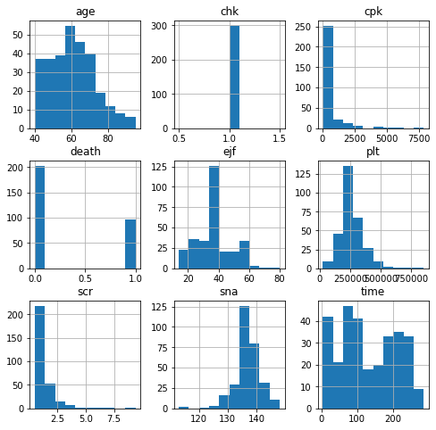
• The age ranged from 40 to 95 years, mean age is 60 years.

• Creatinine phosphokinase- level of CPK enzyme in the blood expressed in mcg/L. it helps in repairing damaged tissues. The normal levels in males are 55–170 mcg/L and in females are 30–135 mcg/L. In this dataset, CPK ranges from 23 to 7861 and the mean is 581.

• Ejection fraction is the percentage of blood leaving the heart at each contraction. It ranges from 14 to 80 and the mean is 38. In a healthy adult, this fraction is 55% and heart failure with reduced ejection fraction implies a value < 40%

• Platelet- This is the platelet count in the blood in kiloplatelets/ml. it ranges from 25,100 to 850,000 with a median of 262,000. A normal person has a platelet count of 150,000–400,000 kiloplatelets/mL of blood.

• Serum creatinine is the level of creatinine in the blood in mg/dl. It is the waste product that is produces dur to muscle break down. The normal levels are between 0.8 to 1.2 mg/dL. Serum creatinine in this dataset ranges from 0.5 to 9.4 with a mean of 1.4

• Serum sodium is the level of sodium in the blood in mEq/L. The normal range is 135-145mEq/L. The serum sodium in this dataset ranges from 113 to 148 with a mean of 136.6

• Time is the follow up period in days, after heart failure. It ranges from 4 to 285 with a mean of 130.3.

hf.shape

#Renaming features

hf = hf.rename(columns={'smoking':'smk',
                        'diabetes':'diab',
                        'anaemia':'anm',
                        'platelets':'plt',
                        'high_blood_pressure':'hbp',
                        'creatinine_phosphokinase':'cpk',
                        'ejection_fraction':'ejf',
                        'serum_creatinine':'scr',
                        'serum_sodium':'sna',
                        'DEATH_EVENT':'death'})
hf['chk'] = 1
hf['sex'] = hf['sex'].apply(lambda x: 'Female' if x==0 else 'Male')
hf['smk'] = hf['smk'].apply(lambda x: 'No' if x==0 else 'Yes')
hf['diab'] = hf['diab'].apply(lambda x: 'No' if x==0 else 'Yes')
hf['anm'] = hf['anm'].apply(lambda x: 'No' if x==0 else 'Yes')
hf['hbp'] = hf['hbp'].apply(lambda x: 'No' if x==0 else 'Yes')
#hf['death'] = hf['death'].apply(lambda x: 'No' if x==0 else 'Yes')
hf.info()

Distribution of the binary features

import matplotlib.pyplot as plt
%matplotlib inline
import seaborn as sns
import plotly.graph_objects as go
palette_ro = ["#ee2f35", "#fa7211", "#fbd600", "#75c731", "#1fb86e", "#0488cf", "#7b44ab"]


fig, ((ax1, ax2, ax3), (ax4, ax5, ax6)) = plt.subplots(2, 3, figsize=(16, 12))

sns.countplot(x="anm", ax=ax1, data=hf,
              palette=palette_ro[3::-3], alpha=0.9)
sns.countplot(x="diab", ax=ax2, data=hf,
              palette=palette_ro[3::-3], alpha=0.9)
sns.countplot(x="hbp", ax=ax3, data=hf,
              palette=palette_ro[3::-3], alpha=0.9)
sns.countplot(x="sex", ax=ax4, data=hf,
              palette=palette_ro[2::3], alpha=0.9)
sns.countplot(x="smk", ax=ax5, data=hf,
              palette=palette_ro[3::-3], alpha=0.9)
sns.countplot(x="death", ax=ax6, data=hf,
              palette=palette_ro[1::5], alpha=0.9)
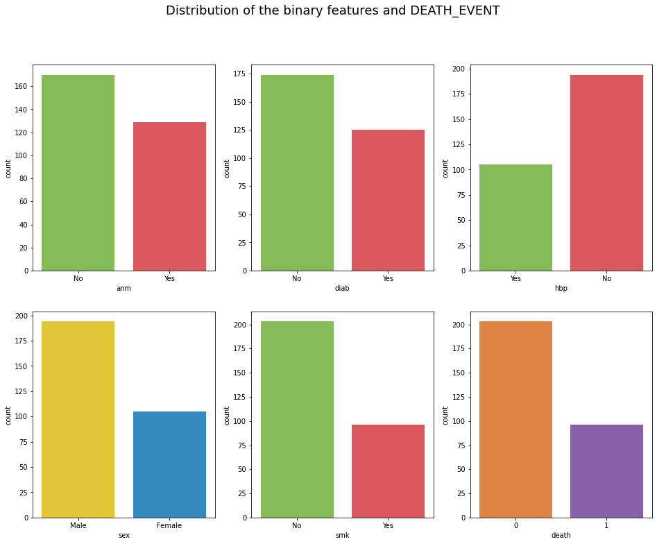
fig.suptitle("Distribution of the binary features and DEATH_EVENT", fontsize=18);

#distribution of numerical features

hf.describe()

numbers = pd.Series(hf.columns)
hf[numbers].hist(figsize = (8, 8))
plt.show();

hf[numbers].skew() 

#age, ejf, and time are normal distributed, cpk, plt, scr are skewed to the left, sna is skewed to the right

pd.crosstab(index=hf['hbp'], columns=hf['death'], values=hf['chk'], aggfunc=np.sum, margins=True)
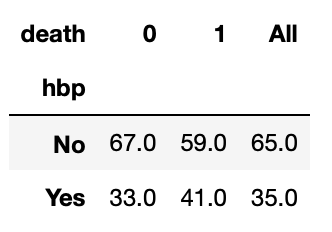
pd.crosstab(index=hf['hbp'], columns=hf['death'], values=hf['chk'], aggfunc=np.sum, margins=True, normalize='columns').round(2)*100

pd.crosstab(index=hf['diab'], columns=hf['death'], values=hf['chk'], aggfunc=np.sum, margins=True)
pd.crosstab(index=hf['diab'], columns=hf['death'], values=hf['chk'], aggfunc=np.sum, margins=True, normalize='columns').round(2)*100

pd.crosstab(index=hf['sex'], columns=hf['death'], values=hf['chk'], aggfunc=np.sum, margins=True)
pd.crosstab(index=hf['sex'], columns=hf['death'], values=hf['chk'], aggfunc=np.sum, margins=True, normalize='columns').round(2)*100

Summary Statistics of Categorical Features

The categorical features are Anemia, Diabetes, High blood pressure, Sex and Smoking.

• 41% of patient who survived had anemia and 48% of patients who died of heart failure had anemia

• 42% of patient who survived had diabetes and 42% of patients who died of heart failure had diabetes.

• 33% of patient who survived had high blood pressure and 41% of patients who died of heart failure had high blood pressure.

• 65% of patient who survived were males and 35% of patients who died of heart failure were females

• 65% of patient who survived were males and 35% of patients who died of heart failure were females.

• 33% of patient who survived smoked and 31% of patients who died of heart failure had no history of smoking.

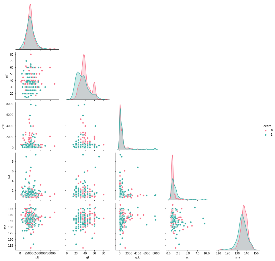
#Exploring relationships between the numerical features

sns.pairplot(hf[['plt', 'ejf', 'cpk', 'scr', 'sna', 'death']], 
             hue='death', palette='husl', corner=True)

# Distribution of target variable
print('% of heart failure patients who died = {}'.format(hf.death.value_counts(normalize=True)[1]))
print('% of heart failure patients who survived = {}'.format(hf.death.value_counts(normalize=True)[0]))

This is an imbalance data

In summary,

• According to the descriptive tables, there is no disparities in sex between people who died and those that survived.
• More people who died had high blood pressure, anemia and smoked compared to those who survived. Those who died from heart failure were older in age, they had higher serum creatinine, serum sodium. They had less ejection fraction and less follow up days compared to those who survived.
• There is no correlation between the features.
• While examining the target variable, I noticed it is a unbalanced data because % of heart failure patient who died = 32% and % of heart failure patients who survived = 68%
• High blood pressure, anemia and smoking, age, higher serum creatinine, serum sodium and ejection fraction may contribute to mortality in those with heart failure

Modeling

In the preprocessing process, scaling of the numerical data was done using the StandardScaler() method in sklearn.preprocessing to scale the values to a m mean of 0 and variance of 1. The numeric data was scaled because they were measured on different scales.

# Scaling data
from sklearn import preprocessing
from sklearn.preprocessing import StandardScaler

#numpy arrays for features and target
x = hf.drop(['time','death'],axis=1).values
y= hf['death'].values

cat_feat = hf[['sex', 'smk', 'diab', 'hbp', 'anm']]
num_feat = hf[['age', 'plt', 'ejf', 'cpk', 'scr', 'sna']]
all1=hf[['sex', 'smk', 'diab', 'hbp', 'anm','age', 'plt', 'ejf', 'cpk', 'scr', 'sna']]

#scaling the numeric features
scaler = StandardScaler()

xscaled= StandardScaler().fit_transform(num_feat)
#scaled_num = pd.DataFrame(scaler.fit_transform(num_feat.values),
                           #columns = num_feat.columns)
#xscaled = pd.concat([cat_feat, scaled_num], axis=1)

xscaled

Because this dataset is an unbalanced one, I used the k- fold cross validation to deal with this imbalance.

The dataset is split into k subsets and the model is trained on the first k-1 subsets and tested on the last kth subset. This process is repeated k times, and the average of the performance measures is calculated (Brownlee, 2020)

A test set and training set is then created from the cross validated samples. I used KFold and cross_validate from sklearn.model_selection to carry out 10-fold cross-validation.

The model used is the supervised classification model logistic regression, random forest and Naïve bayes. They are good for understanding unbalance target models.

# Training and Test set creation- 80:20
from sklearn.model_selection import train_test_split

x_train, x_test, y_train, y_test = train_test_split(xscaled, y, test_size=0.2, random_state=1)

Logistics Regression

from sklearn.metrics import accuracy_score
from sklearn.metrics import classification_report
from sklearn.metrics import confusion_matrix


from sklearn.linear_model import LogisticRegression
lr = LogisticRegression()
lr.fit(x_train,y_train)
pred = lr.predict(x_test)

print("Confusion Matrix : \n\n" , confusion_matrix(pred,y_test), "\n")
print("Classification Report : \n\n" , classification_report(pred,y_test),"\n")

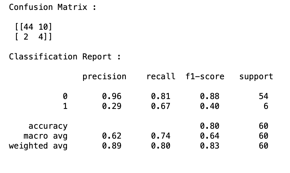
Accuracy=80 sens=67 spe=96

accuracy_score(pred,y_test)

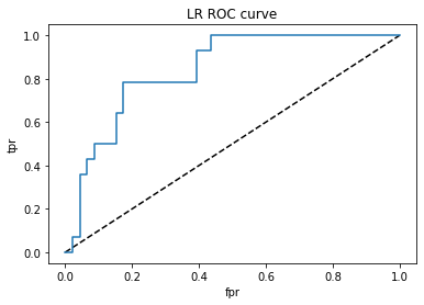
# Find and plot AUC
from sklearn.metrics import roc_curve, roc_auc_score


y_pred_proba=lr.predict_proba(x_test)[:,1]
fpr, tpr, thresholds = roc_curve(y_test, y_pred_proba)

import matplotlib.pyplot as plt

plt.plot([0,1],[0,1],'k--')
plt.plot(fpr,tpr, label='Knn')
plt.xlabel('fpr')
plt.ylabel('tpr')
plt.title('LR ROC curve')
plt.show()

roc_auc_score(y_test,y_pred_proba)

Logistics Regretion with Cross Validation

#10 fold cross validation

from sklearn.datasets import make_classification
from sklearn.model_selection import KFold
# generate 2 class dataset
x, y = make_classification(n_samples=299, n_classes=2, weights=[0.80, 0.20], flip_y=0, random_state=1)
kfold = KFold(n_splits=10, shuffle=True, random_state=1)
# enumerate the splits and summarize the distributions
for train_ix, test_ix in kfold.split(x):
    # select rows
    train_x, test_x = x[train_ix], x[test_ix]
    train_y, test_y = y[train_ix], y[test_ix]
    # summarize train and test composition
    train_0, train_1 = len(train_y[train_y==0]), len(train_y[train_y==1])
    test_0, test_1 = len(test_y[test_y==0]), len(test_y[test_y==1])


    

from sklearn.linear_model import LogisticRegression
from sklearn.model_selection import cross_validate
lr = LogisticRegression()

scores= cross_validate(lr, x, y, cv=kfold, scoring=('accuracy','balanced_accuracy', 'precision', 'recall', 'roc_auc'), return_train_score = True)

print("Logistic Regression Accuracy:", "{:.2f}%".format(scores['test_accuracy'].mean()*100))
print("Logistic Regression Precision :", "{:.2f}%".format(scores['test_precision'].mean()*100))
print("Logistic Regression Recall :", "{:.2f}%".format(scores['test_recall'].mean()*100))

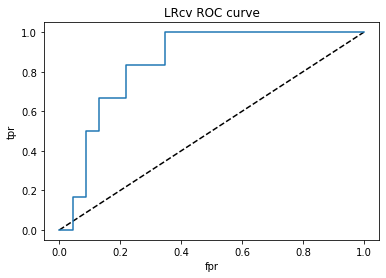
# Find and plot AUC after CV
from sklearn.metrics import roc_curve, roc_auc_score

lr.fit(train_x,train_y)
y_pred_proba=lr.predict_proba(test_x)[:,1]
fpr, tpr, thresholds = roc_curve(test_y, y_pred_proba)

import matplotlib.pyplot as plt

plt.plot([0,1],[0,1],'k--')
plt.plot(fpr,tpr, label='Knn')
plt.xlabel('fpr')
plt.ylabel('tpr')
plt.title('LRcv ROC curve')
plt.show()

roc_auc_score(test_y,y_pred_proba)

Logistics Regression result

Running a logistic regressing model on the 12 features yielded an accuracy of 80%, sensitivity of 67% and specificity of 96%. These are good values which indicates that those 12 features are an optimum number of features.

Running a logistics regression model after 10-fold cross validation, the model with 12 features yielded accuracy of 88%, sensitivity of 65% and specificity of 72%.

Random forest

from sklearn.ensemble import RandomForestClassifier
rf = RandomForestClassifier(n_estimators=100, random_state=0)
rf.fit(train_x,train_y)
print("Accuracy on training set: {:.3f}".format(rf.score(train_x, train_y)))
print("Accuracy on test set: {:.3f}".format(rf.score(test_x, test_y)))
pred = rf.predict(test_x)

# Let's tune the min_samples_split based on gridserachCV

#import GridSearchCV
from sklearn.model_selection import GridSearchCV

# the parameter to be tuned is max_depth

param_grid_split = {'min_samples_split':np.arange(10,50,5)} # get a list of minimum samples split

tree = RandomForestClassifier(random_state=0)

tree_cv_split= GridSearchCV(tree,param_grid_split,cv=10)

tree_cv_split.fit(train_x, train_y)

# Let's tune the max_depth based on gridserachCV

#import GridSearchCV
from sklearn.model_selection import GridSearchCV

# the parameter to be tuned is max_depth

param_grid_depth = {'max_depth':np.arange(1,15)} # get a list of depth parameters

tree = RandomForestClassifier(random_state=0)

tree_cv_depth= GridSearchCV(tree,param_grid_depth,cv=10)

tree_cv_depth.fit(train_x, train_y)

tree_cv_split.best_params_

tree_cv_depth.best_params_

# lets select the best parameters and run the classifier again.

rf1 = RandomForestClassifier(max_depth=7, min_samples_split=10, n_estimators=100, random_state=0, oob_score=bool)
rf1.fit(train_x,train_y)
print("Accuracy on training set: {:.3f}".format(rf1.score(train_x, train_y)))
print("Accuracy on test set: {:.3f}".format(rf1.score(test_x, test_y)))

y_pred =rf1.predict(test_x)

from sklearn.metrics import classification_report

print(classification_report(test_y,y_pred))

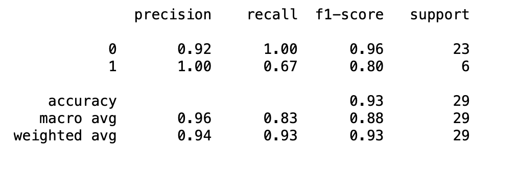
acc-93% sen-67% spe-92%

print("Feature importances:\n{}".format(rf1.feature_importances_))

important_features_dict = {}
for x,i in enumerate(rf1.feature_importances_):
    important_features_dict[x]=i


important_features_list = sorted(important_features_dict,
                                 key=important_features_dict.get,
                                 reverse=True)

print ('Most important features: %s' %important_features_list)

featureImpList= []

for feat, importance in zip(all1, rf1.feature_importances_):  
    temp = [feat, importance*100]
    featureImpList.append(temp)

# create a dataframe

fT_df = pd.DataFrame(featureImpList, columns = ['Feature', 'Importance'])

# sort the values

fT_df_sorted = fT_df.sort_values('Importance', ascending = False)
print (fT_df_sorted)

accuracy_score(test_y,y_pred)

# Find and plot AUC
from sklearn.metrics import roc_curve, roc_auc_score


y_pred_proba=rf1.predict_proba(test_x)[:,1]
fpr, tpr, thresholds = roc_curve(test_y, y_pred_proba)

import matplotlib.pyplot as plt

plt.plot([0,1],[0,1],'k--')
plt.plot(fpr,tpr, label='Knn')
plt.xlabel('fpr')
plt.ylabel('tpr')
plt.title('Random forest ROC curve')
plt.show()

roc_auc_score(test_y,y_pred_proba)

Random forest Result

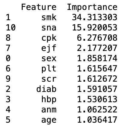
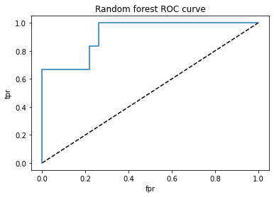
Initially the accuracy on the testing set was 0.9 and the accuracy on the training set was 1.0. After the grid searchcv was ran, the parameters were tunes to a minimum sample split of 10 and the tree cv mac depth of 7. This resulted in a training accuracy of 0.99 and a test accuracy of 0.93. the classification report showed an accuracy of 93%, sensitivity of 67% and specificity of 92%. The important features according to the random forest are smk, sna,cpk,hbp, sex, scr, ejf, plt, age, diab and anm.

Naive bayes

from sklearn.naive_bayes import GaussianNB
gnb=GaussianNB()
gnb.fit(train_x,train_y)
gnb_predict=gnb.predict(test_x)
gnb.score(test_x,test_y)

from sklearn.metrics import confusion_matrix
confusion_matrix(test_y,gnb_predict)
pd.crosstab(test_y,gnb_predict,margins=True)

accuracy_score(test_y,gnb_predict)

from sklearn.metrics import classification_report

print(classification_report(test_y,gnb_predict))

acc-83% sen-67% spe-91%

# Find and plot AUC
from sklearn.metrics import roc_curve, roc_auc_score


y_pred_proba=gnb.predict_proba(test_x)[:,1]
fpr, tpr, thresholds = roc_curve(test_y, y_pred_proba)

import matplotlib.pyplot as plt

plt.plot([0,1],[0,1],'k--')
plt.plot(fpr,tpr, label='Knn')
plt.xlabel('fpr')
plt.ylabel('tpr')
plt.title('Naive Bayes ROC curve')
plt.show()

roc_auc_score(test_y,y_pred_proba)

Naïve Bayes Result

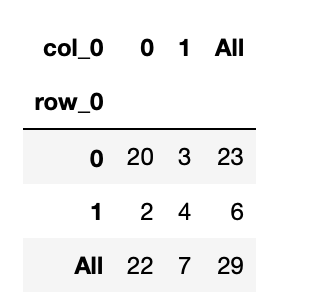
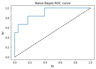
The accuracy for the naïve bayes is 83%, sensitivity is 67% and specificity is 91%. AUC score is 90%

Discussion

The model evaluation technique I used was accuracy, sensitivity and specificity score. The most important is the sensitivity because it will be beneficial for a health care provider to accurately predict the patient who will have a bad outcome to avert it in a timely manner. We are interested in how many deaths will be correctly predicted.

Random forest is considered as an advanced machine learning technique, especially if the dataset is imbalanced or has categorical features. It had the highest accuracy compared to naïve bayes and logistics regression. Based on sensitivity, the random forest performed best. This means that more deaths will be accurately predicted.

Conclusion

The results show that you can successfully predict the outcome of heart failure is possible using a combination of laboratory and clinical criteria. In clinical practice the naïve bayes method will be more useful and it has a higher specificity, high accuracy and specificity. This is encouraging in clinical practice and in rural areas where there might be poor access to health care services. In the absence of expensive laboratory tests, the physician may be able to predict the survival outcome of heart failure using clinical and examination findings.